Chapter 4 Supervised Learning — Regression
4.1 Historical notes
Regression is an important technique in statistics and machine learning. It was first introduced by Sir Francis Galton in the 19th century. He used it to study the relationship between the heights of fathers and their sons. The term “regression” was coined by Galton to describe the tendency of the heights of sons to “regress” towards the mean height of the population. For us, the general idea is to predict a continuous value from a set of input variables.
As we have already seen, metrics for regression are different from those for classification. Historically, machine learning techniques for regression have focused on getting as close as possible to the target variable with little regard for prediction uncertainty. This is changing as we move towards more complex models that can provide a measure of uncertainty in their predictions.
4.2 Running example
Like in the previous chapter, we will use two well-known data sets to illustrate regression techniques. The first is the Boston housing data set, which contains information about housing in the Boston area. The target variable is the median value of owner-occupied homes in thousands of dollars. The data set contains 506 observations on 14 variables. The second data set is the Auto MPG data set, which contains information about cars. The target variable is the miles per gallon (MPG) of the car. The data set contains 398 observations on 9 variables.
In both cases, it is trivial to set up a linear regression model in R.
# load in the data
library(MASS)
data(Boston)
data(mtcars)

# standardise the data to aid interpretation
Boston <- as.data.frame(scale(Boston))
mtcars <- as.data.frame(scale(mtcars))

# linear regression
lm.fit.Boston <- lm(medv ~ ., data = Boston)
summary(lm.fit.Boston)
##
## Call:
## lm(formula = medv ~ ., data = Boston)
##
## Residuals:
## Min 1Q Median 3Q Max
## -1.69559 -0.29680 -0.05633 0.19322 2.84864
##
## Coefficients:
## Estimate Std. Error t value Pr(>|t|)
## (Intercept) -2.211e-16 2.294e-02 0.000 1.000000
## crim -1.010e-01 3.074e-02 -3.287 0.001087 **
## zn 1.177e-01 3.481e-02 3.382 0.000778 ***
## indus 1.534e-02 4.587e-02 0.334 0.738288
## chas 7.420e-02 2.379e-02 3.118 0.001925 **
## nox -2.238e-01 4.813e-02 -4.651 4.25e-06 ***
## rm 2.911e-01 3.193e-02 9.116 < 2e-16 ***
## age 2.119e-03 4.043e-02 0.052 0.958229
## dis -3.378e-01 4.567e-02 -7.398 6.01e-13 ***
## rad 2.897e-01 6.281e-02 4.613 5.07e-06 ***
## tax -2.260e-01 6.891e-02 -3.280 0.001112 **
## ptratio -2.243e-01 3.080e-02 -7.283 1.31e-12 ***
## black 9.243e-02 2.666e-02 3.467 0.000573 ***
## lstat -4.074e-01 3.938e-02 -10.347 < 2e-16 ***
## ---
## Signif. codes: 0 '***' 0.001 '**' 0.01 '*' 0.05 '.' 0.1 ' ' 1
##
## Residual standard error: 0.516 on 492 degrees of freedom
## Multiple R-squared: 0.7406, Adjusted R-squared: 0.7338
## F-statistic: 108.1 on 13 and 492 DF, p-value: < 2.2e-16##
## Call:
## lm(formula = mpg ~ ., data = mtcars)
##
## Residuals:
## Min 1Q Median 3Q Max
## -0.57254 -0.26620 -0.01985 0.20230 0.76773
##
## Coefficients:
## Estimate Std. Error t value Pr(>|t|)
## (Intercept) 9.929e-18 7.773e-02 0.000 1.0000
## cyl -3.302e-02 3.097e-01 -0.107 0.9161
## disp 2.742e-01 3.672e-01 0.747 0.4635
## hp -2.444e-01 2.476e-01 -0.987 0.3350
## drat 6.983e-02 1.451e-01 0.481 0.6353
## wt -6.032e-01 3.076e-01 -1.961 0.0633 .
## qsec 2.434e-01 2.167e-01 1.123 0.2739
## vs 2.657e-02 1.760e-01 0.151 0.8814
## am 2.087e-01 1.703e-01 1.225 0.2340
## gear 8.023e-02 1.828e-01 0.439 0.6652
## carb -5.344e-02 2.221e-01 -0.241 0.8122
## ---
## Signif. codes: 0 '***' 0.001 '**' 0.01 '*' 0.05 '.' 0.1 ' ' 1
##
## Residual standard error: 0.4397 on 21 degrees of freedom
## Multiple R-squared: 0.869, Adjusted R-squared: 0.8066
## F-statistic: 13.93 on 10 and 21 DF, p-value: 3.793e-07The summaries here give us the adjusted R-squared, amongst other things. It is interesting to consider the model coefficients in these models and to look at which are significantly different from zero. We can also calculate the other performance measures that we met in the earlier chapter using the fitted models.
| Boston | Auto MPG | |
|---|---|---|
| MSE | 0.26 | 0.13 |
| RMSE | 0.51 | 0.36 |
| MAE | 0.36 | 0.29 |
| MSLE | NaN | NaN |
| MAPE | 2.51 | 0.64 |
You will note that some of these return NaN values. This is because the target variable contains zeros. We can remove these from the data set to avoid this issue or think more carefully about which metric is appropriate for the problem at hand. You will also note that, in isolation, these metrics are not particularly informative. They are useful for comparing models, but not for understanding the quality of the model.
4.3 Regularised Regression
As discussed in the section on overfitting, regularisation is a fundamental technique used to prevent models from becoming overly complex and generalising poorly to new data. The core idea behind regularisation is to add a penalty term to the loss function that discourages large parameter values, effectively trading off some training accuracy for better generalisation performance.
Before going into specific regularisation techniques, it is important to revisit and understand the bias-variance trade-off that underlies regularisation. When we fit a model:
- Bias refers to the error introduced by approximating a complex real-world problem with a simplified model
- Variance refers to the sensitivity of the model to small changes in the training data
- Irreducible error is the noise inherent in the problem that cannot be eliminated
Regularisation techniques deliberately introduce some bias to significantly reduce variance, often resulting in lower total error. This is particularly valuable when we have: - Limited training data, - Many variables relative to observations, - Multicollinearity among predictors.
4.3.1 Types of Regularisation
There are three main types of regularisation for linear regression: L1 (Lasso), L2 (Ridge), and Elastic Net (a combination of both). Each has distinct properties and use cases.
- Ridge Regression: Use when you believe most variables are relevant but want to prevent overfitting. Ridge keeps all variables but shrinks their coefficients toward zero.
- Lasso Regression: Use when you suspect many variables are irrelevant and want automatic Variable selection. Lasso can set coefficients exactly to zero.
- Elastic Net: Use when you have groups of correlated variables. Elastic Net tends to select groups of correlated variables together, unlike Lasso, which may arbitrarily select one from a correlated group.
4.3.2 Mathematical Foundation
Recall that ordinary least squares (OLS) regression finds coefficients by minimising the mean squared error:
\[ \text{Loss}_{\text{OLS}} = \sum_{i=1}^{n} (y_i - \widehat{y}_i)^2 = ||\mathbf{y} - X\beta||_2^2 \]
The closed-form solution is: \[ \widehat{\beta}_{\text{OLS}} = (X^T X)^{-1} X^T \mathbf{y} \]
When using regularised regression, it is essential to standardise both the predictors and response variable because regularisation penalties are sensitive to the scale of variables. Standardisation ensures that penalties are applied equally across all variables.
4.3.2.1 Ridge Regression (L2 Regularisation)
Ridge regression adds an L2 penalty term to the loss function that penalises the sum of squared coefficients:
\[ \text{Loss}_{\text{Ridge}} = ||\mathbf{y} - X\beta||_2^2 + \lambda ||\beta||_2^2 = \sum_{i=1}^{n} (y_i - \widehat{y}_i)^2 + \lambda \sum_{j=1}^{p} \beta_j^2 \]
The closed-form solution becomes: \[ \widehat{\beta}_{\text{Ridge}} = \left(X^{T} X + \lambda I\right)^{-1} X^{T} \mathbf{y} \]
Ridge regression is particularly effective at handling multicollinearity, a common issue where two or more predictor variables are highly correlated. In such scenarios, the design matrix \(X\) becomes ill-conditioned, meaning the \(X^TX\) matrix is close to singular and difficult to invert. This leads to ordinary least squares (OLS) coefficient estimates that are highly sensitive to small changes in the data, resulting in large variances and instability. By adding the regularisation term \(\lambda I\) to the \(X^TX\) matrix, ridge regression ensures that the matrix \(\left(X^{T} X + \lambda I\right)\) is invertible and well-conditioned, regardless of the correlation among the predictors. This process stabilises the estimates and reduces their variance, producing more reliable and robust coefficients than ordinary least squares in the presence of multicollinearity.
Key Properties: - Never sets coefficients exactly to zero - Shrinks coefficients of correlated variables toward each other - Computationally efficient (closed-form solution) - From a Bayesian perspective, equivalent to placing a Gaussian prior on coefficients
Geometric Interpretation: The L2 constraint creates a circular constraint region. The optimal solution occurs where the elliptical contours of the loss function touch this circular constraint.
4.3.2.2 Lasso Regression (L1 Regularisation)
Lasso (Least Absolute Shrinkage and Selection Operator) regression uses an L1 penalty that penalises the sum of absolute values of coefficients:
\[ \text{Loss}_{\text{Lasso}} = ||\mathbf{y} - X\beta||_2^2 + \lambda ||\beta||_1 = \sum_{i=1}^{n} (y_i - \widehat{y}_i)^2 + \lambda \sum_{j=1}^{p} |\beta_j| \]
The optimisation problem is: \[ \widehat{\beta}_{\text{Lasso}} = \text{argmin}_{\beta} \left( ||\mathbf{y} - X\beta||_2^2 + \lambda ||\beta||_1 \right) \]
Key Properties: - Can set coefficients exactly to zero (automatic Variable selection), - Tends to select one Variable from a group of correlated variables, - No closed-form solution; requires iterative algorithms (coordinate descent), - From a Bayesian perspective, equivalent to placing a Laplace prior on coefficients.
Geometric Interpretation: The L1 constraint creates a diamond-shaped constraint region. The corners of this diamond lie on the coordinate axes, which is why Lasso can produce exactly zero coefficients.
4.3.3 Elastic Net Regression
Elastic Net combines L1 and L2 penalties, providing a balance between Ridge and Lasso:
\[ \text{Loss}_{\text{Elastic Net}} = ||\mathbf{y} - X\beta||_2^2 + \lambda \left( \alpha ||\beta||_1 + (1-\alpha) ||\beta||_2^2 \right) \]
where \(\alpha \in [0,1]\) controls the balance between L1 and L2 penalties: - \(\alpha = 0\): Pure Ridge regression, - \(\alpha = 1\): Pure Lasso regression, - \(0 < \alpha < 1\): Combination of both penalties.
Key Properties: - Combines Variable selection (L1) with coefficient shrinkage (L2) - Handles groups of correlated variables better than Lasso - Particularly useful when \(p > n\) (more variable than observations)
4.3.4 Hyperparameter Selection
The regularisation strength \(\lambda\) (and \(\alpha\) for Elastic Net) are hyperparameters that must be chosen carefully. The most common approach is \(k\)-fold cross-validation:
- Split training data into \(k\) folds.
- For each candidate hyperparameter value:
- Train on \(k-1\) folds,
- Validate on the remaining fold,
- Repeat for all folds.
- Select hyperparameters that minimise average validation error.
Grid Search can be used to search over combinations of hyperparameters systematically. Of course, this can be computationally expensive, especially for large datasets or complex models.
Example
We will demonstrate the strengths and weaknesses of each regularisation method using a carefully constructed synthetic dataset.
# Load required libraries
library(glmnet)
library(caret)
library(ggplot2)
library(dplyr)
library(tidyr)
library(gridExtra)

# Set seed for reproducibility
set.seed(42)

# Create a synthetic dataset with known structure
n <- 200  # number of observations
p <- 50   # number of variables

# Generate correlated predictors
X <- matrix(rnorm(n * p), n, p)

# Add correlation structure: variables 1-5 are highly correlated
for(i in 2:5) {
  X[, i] <- 0.7 * X[, 1] + 0.3 * X[, i]
}

# variable 6-10 are moderately correlated
for(i in 7:10) {
  X[, i] <- 0.5 * X[, 6] + 0.5 * X[, i]
}

# True coefficient structure:
# - variable 1, 6, 11, 16, 21 have large effects (truly important)
# - variable 2-5, 7-10 have small effects (correlated groups)
# - Remaining variables have zero effect (noise)
true_beta <- rep(0, p)
true_beta[c(1, 6, 11, 16, 21)] <- c(3, 2.5, 2, 1.5, 1)  # Important variable
true_beta[2:5] <- 0.5   # Correlated with Variable 1
true_beta[7:10] <- 0.3  # Correlated with Variable 6

# Generate response with noise
y <- X %*% true_beta + rnorm(n, 0, 0.5)

# Split into training and test sets
train_idx <- sample(1:n, 0.7 * n)
X_train <- X[train_idx, ]
y_train <- y[train_idx]
X_test <- X[-train_idx, ]
y_test <- y[-train_idx]

# Standardise the data (crucial for regularisation!)
X_train_scaled <- scale(X_train)
X_test_scaled <- scale(X_test,
                       center = attr(X_train_scaled, "scaled:center"),
                       scale = attr(X_train_scaled, "scaled:scale"))
y_train_scaled <- scale(y_train)[, 1]
y_test_scaled <- scale(y_test,
                       center = attr(scale(y_train), "scaled:center"),
                       scale = attr(scale(y_train), "scaled:scale"))[, 1]

# Need to standardise the beta coeffs for later comparison
true_beta_scaled <- true_beta / attr(scale(y_train), "scaled:scale")

# Create combined data frames for training and test sets
X_train_scaled <- as.data.frame(X_train_scaled)
X_test_scaled <- as.data.frame(X_test_scaled)
y_train_scaled <- as.data.frame(y_train_scaled)
y_test_scaled <- as.data.frame(y_test_scaled)
# Rename columns for clarity
colnames(X_train_scaled) <- paste0("X", 1:p)
colnames(X_test_scaled) <- paste0("X", 1:p)
# Combine predictors and response for training and test sets
train_data <- cbind(y_train_scaled, X_train_scaled)
test_data <- cbind(y_test_scaled, X_test_scaled)

cat("Dataset created with:\n")
## Dataset created with:## - 5 truly important variable## - 2 groups of correlated variable (4 variable each)## - 37 noise variable## - Training set: 140 observations## - Test set: 60 observationsFor ordinary least squares (OLS) regression, we can use the lm function in R. For Ridge, Lasso, and Elastic Net regression, we will use the glmnet package. The glmnet package provides efficient implementations of these regularised regression techniques.
# 1. Ordinary Least Squares (OLS)
ols_model <- lm(y_train_scaled ~ .,
                data = train_data)
ols_pred <- predict(ols_model,
                    newdata = test_data)
ols_mse <- mean((y_test_scaled[,1] - ols_pred)^2)

# 2. Ridge Regression
ridge_cv <- cv.glmnet(x = as.matrix(X_train_scaled),
                     y = y_train_scaled[,1],
                      alpha = 0, nfolds = 10)
ridge_pred <- predict(ridge_cv, s = "lambda.min",
                      newx = as.matrix(X_test_scaled))
ridge_mse <- mean((y_test_scaled[,1] - ridge_pred)^2)
ridge_coef <- coef(ridge_cv, s = "lambda.min")[-1]  # Remove intercept

# 3. Lasso Regression
lasso_cv <- cv.glmnet(x = as.matrix(X_train_scaled),
                     y = y_train_scaled[,1], alpha = 1, nfolds = 10)
lasso_pred <- predict(lasso_cv, s = "lambda.min",
                      newx = as.matrix(X_test_scaled))
lasso_mse <- mean((y_test_scaled[,1] - lasso_pred)^2)
lasso_coef <- coef(lasso_cv, s = "lambda.min")[-1]  # Remove intercept

# 4. Elastic Net Regression
elastic_grid <- expand.grid(alpha = seq(0.1, 0.9, by = 0.1),
                            lambda = seq(0.001, 0.1, length = 20))

elastic_model <- train(x = as.matrix(X_train_scaled),
                     y = y_train_scaled[,1],
                       method = "glmnet",
                       tuneGrid = elastic_grid,
                       trControl = trainControl(method = "cv", number = 10),
                       standardise = FALSE)  # Already standardised

elastic_pred <- predict(elastic_model, X_test_scaled)
elastic_mse <- mean((y_test_scaled[,1] - elastic_pred)^2)
elastic_coef <- coef(elastic_model$finalModel, s = elastic_model$bestTune$lambda)[-1]| Method | Test_MSE | Non_zero_coef | Lambda |
|---|---|---|---|
| OLS | 0.0145 | 50 | NA |
| Ridge | 0.0222 | 50 | 0.0745 |
| Lasso | 0.0127 | 18 | 0.0103 |
| Elastic Net | 0.0127 | 19 | 0.0114 |
Elastic Net optimal alpha: 0.9
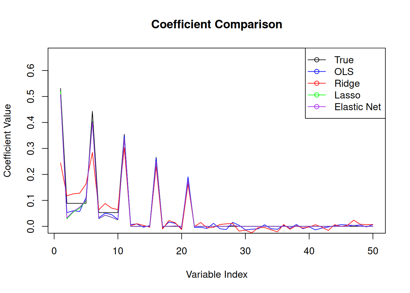
With the ridge regression coefficients, we can see the effect of the regularisation being too strong. The coefficients are shrunk towards zero, but not set to zero. This is the expected behaviour of ridge regression. The lasso regression coefficients, on the other hand, show that some coefficients are set to zero, which is the expected behaviour of lasso regression. The elastic net coefficients show a combination of both ridge and lasso regression, with some coefficients set to zero and others shrunk towards zero.
Example
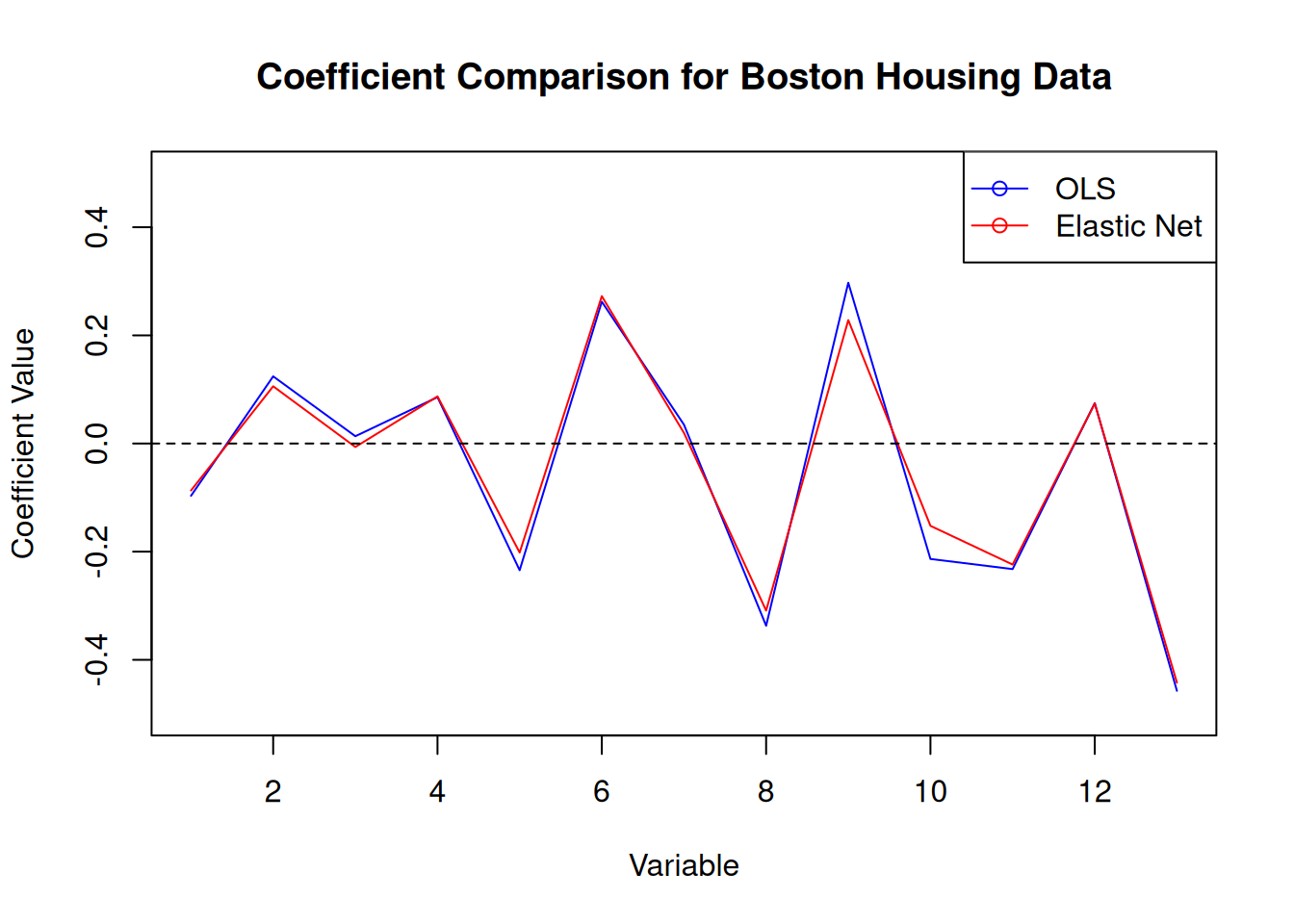
We will now fit a regularised regression model to the Boston housing data set again using the glmnet package.
# Load the Boston data set
library(MASS)
data(Boston)
# Standardise the data
Boston <- as.data.frame(scale(Boston))
# Set up train and test sets
set.seed(123)
trainIndex <- sample(1:nrow(Boston), 0.8 * nrow(Boston))
trainBoston <- Boston[trainIndex,]
testBoston <- Boston[-trainIndex,]

# OLS for coeff comparison
ols.fit.Boston <- lm(medv ~ ., data = trainBoston)
ols.pred <- predict(ols.fit.Boston, newdata = testBoston)
ols.MLE <- mean((ols.pred - testBoston$medv)^2)

# Elastic Net Regression
elastic_grid <- expand.grid(alpha = seq(0.1, 0.9, by = 0.1),
                            lambda = seq(0.001, 0.1, length = 20))
elastic.fit.Boston <- train(medv ~ .,
                             data = trainBoston,
                             method = "glmnet",
                             tuneGrid = elastic_grid,
                             trControl = trainControl(method = "cv", number = 10),
                             standardise = FALSE)  # Already standardised
elastic.pred <- predict(elastic.fit.Boston, newdata = testBoston)
elastic.MSE <- mean((elastic.pred - testBoston$medv)^2)
In this case, we get a regularisation parameter of 0.0166 and an optimal alpha of 0.1. The MSE for the elastic net model is 0.28, which is slightly lower than the MSE for the OLS model of 0.28.
4.4 \(k\)-nearest neighbours
Like in the classification setting, we can use \(k\)-nearest neighbours for regression. The idea is exactly the same: we predict the target variable by averaging the values of the \(k\)-nearest neighbours. The updated algorithm is given by
- Calculate the distance between the test point and all the training points.
- Sort the distances and determine the \(k\)-nearest neighbours.
- Average the target variable of the \(k\)-nearest neighbours.
Again, the choice of \(k\) is important in \(k\)-nearest neighbours. A small value of \(k\) will result in a model that is sensitive to noise, while a large value of \(k\) will result in a model that is biased. The choice of \(k\) will depend on the problem at hand and the amount of noise in the data. More formally, the mathematical representation of the \(k\)-nearest neighbours algorithm is \[ \widehat{y} = \frac{1}{k} \sum_{i=1}^{k} y_i \] where \(\widehat{y}\) is the predicted value, \(k\) is the number of neighbours, and \(y_i\) is the target variable of the \(i\)-th neighbour.
Step 2 of the algorithm can be computationally challenging with large training sets. The knn package in R uses a data structure called a k-d tree to speed up the calculation of the distances between the test point and the training points. The \(k\)-d tree is a binary tree that is used to partition the input space into regions. The \(k\)-d tree is built by recursively splitting the input space along the dimensions of the input variables. The \(k\)-d tree is used to find the \(k\)-nearest neighbours by traversing the tree and only considering the regions that contain the \(k\)-nearest neighbours.
The final predictions can be thought of as a piecewise constant function over the input space defined by the training data. The different prediction values sit on a Voronoi tessellation whose tiles are determined by the training data. The idea behind \(k\)-nearest neighbours is related to the idea of stacking that we will meet in the next section. Stacking uses the predictions of multiple models to make a final prediction. In the case of \(k\)-nearest neighbours, the prediction “models” are the \(k\)-nearest neighbours themselves.
Example
We fit a \(k\)-nearest neighbours model to the Boston data set using the knn package within caret.
set.seed(123)
# Set up train and test sets
trainIndex <- sample(1:nrow(Boston), 0.8 * nrow(Boston))
trainBoston <- Boston[trainIndex,]
testBoston <- Boston[-trainIndex,]

# Fit the model
knn.fit.Boston <- train(medv ~ .,
data = Boston,
method = "knn",
trControl = trainControl(method = "cv",
number = 10))

# Predictions
knn.pred <- predict(knn.fit.Boston, testBoston)
Figure 4.3 shows the model performance in terms of the actual and predicted values.
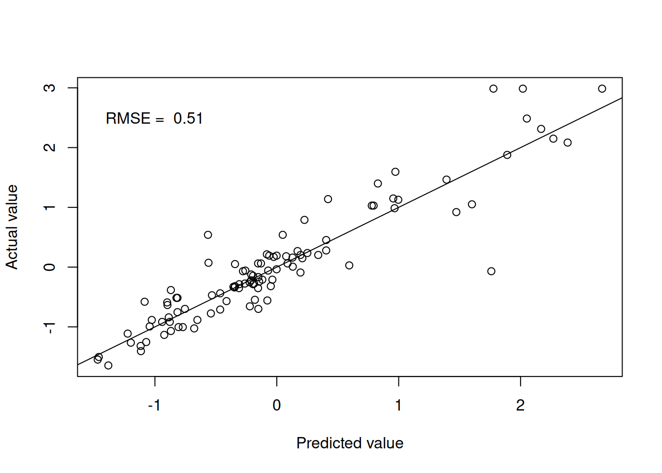
Figure 4.1: k-nearest neighbours predictions
We can extend the \(k\)-nearest neighbours model to include a weighting term in the prediction. The weighting term is a function of the distance between the test point and the training points. The idea is to give more weight to the training points that are closer to the test point. The weighted \(k\)-nearest prediction is calculated using
\[
\widehat{y} = \frac{\sum_{i=1}^{k} w_i y_i}{\sum_{i=1}^{k} w_i}
\]
where \(w_i\) is the weight of the \(i\)-th neighbour. The weights are typically calculated using the inverse of the distance between the test point and the training points. The weighted \(k\)-nearest neighbours model is implemented in the kknn package in R.
set.seed(123)
# Fit the model
kknn.fit.Boston <- train(medv ~ .,
data = Boston,
method = "kknn",
trControl = trainControl(method = "cv",
number = 10))

# Predictions
kknn.pred <- predict(kknn.fit.Boston, testBoston)
Figure 4.4 shows the model performance in terms of the actual and predicted values utilising the distance weights.
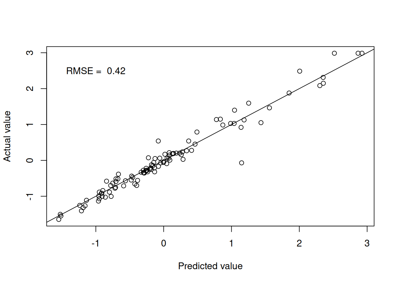
Figure 4.2: Weighted k-nearest neighbours predictions
4.5 Decision trees
Decision trees provide yet another non-parametric regression technique that is based on recursive partitioning of the input space that work the same way as in the classification setting. The idea is to split the input space into regions and fit a simple model to each region. The model is trained by recursively splitting the input space into regions until a stopping criterion is met. The stopping criterion can be based on the number of observations in a region, the depth of the tree, or the impurity of the regions. The impurity of a region is a measure of how well the target variable is predicted by the model in that region. The impurity can be measured using the mean squared error, the mean absolute error, or the mean squared logarithmic error.
In the standard implementation, the model is simply the mean of the target variable in the region. The final model is therefore a multidimensional step function over the space of explanatory variables.
Example
Let’s see it in action for the mtcars data set.
set.seed(123)
# Set up train and test sets
trainIndex <- createDataPartition(mtcars$mpg, p = 0.8,
list = FALSE)
trainMtcars <- mtcars[trainIndex,]
testMtcars <- mtcars[-trainIndex,]

# Fit the model
tree.fit.mtcars <- train(mpg ~ .,
data = mtcars,
method = "rpart",
trControl = trainControl(method = "cv",
number = 10))

# Predictions
tree.pred <- predict(tree.fit.mtcars,
testMtcars)
Figures 4.5 and 4.6 show the model performance in terms of the actual and predicted values and the fitted decision tree. The model here is extremely simple with only two splits. Essentially, the model provides just three values for the mean behaviour of the target variable. This is to be expected given the small number of observations in the data set.
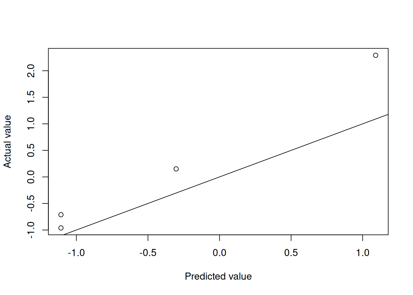
Figure 4.3: Decision tree predictions
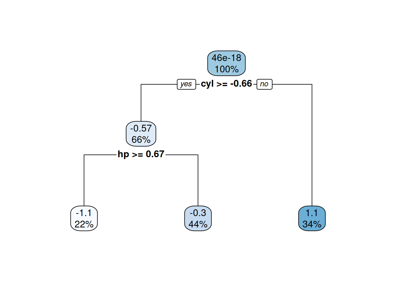
Figure 4.4: Fitted decision tree
4.6 Multivariate Adaptive Regression Splines
The Multivariate Adaptive Regression Spline (MARS) method is a non-parametric regression technique that is based on piecewise linear functions. MARS models are built by recursively partitioning the input space into regions and fitting a linear function to each region. This should sound familiar as it is the same idea as decision trees. The difference is that the MARS model is built from simple linear functions, while the decision tree model is built from constant functions.
We write the MARS model in terms of hinge functions, which are piecewise linear functions that are used to create the piecewise linear functions in the MARS model: \[ f({\mathbf{x}}) = \beta_0 + \sum_{j=1}^{m} \beta_j h_j({\mathbf{x}}), \] where the \(\beta_j\) are the model parameters and the \(h_j({\mathbf{x}})\) are the hinge functions. The hinge functions are defined as \[ h_j({\mathbf{x}}) = \max(0, x_k - c_j) \quad \text{or} \quad \max(0, c_j - x_k), \] where \(x_k\) is one of the input variables and \(c_j\) is the knot point. The “or” here allows us to have functions with negative or positive gradients. The MARS model is built by adding hinge functions to the model and selecting the most important hinge functions. This means that we need to estimate the location of the knot points and the coefficients of the hinge functions. In practice, the knot locations are determined in a manner akin to the decision tree algorithm.
The MARS model is often trained by considering reductions in RMSE. At each stage of the algorithm, the model is trained by adding a hinge function that reduces the RMSE the most. The algorithm is stopped when the RMSE is no longer reduced by adding a hinge function.
The MARS model has the advantage of being interpretable because the model is built from simple linear functions. Figure 4.7 shows an example of the MARS model in one dimension.
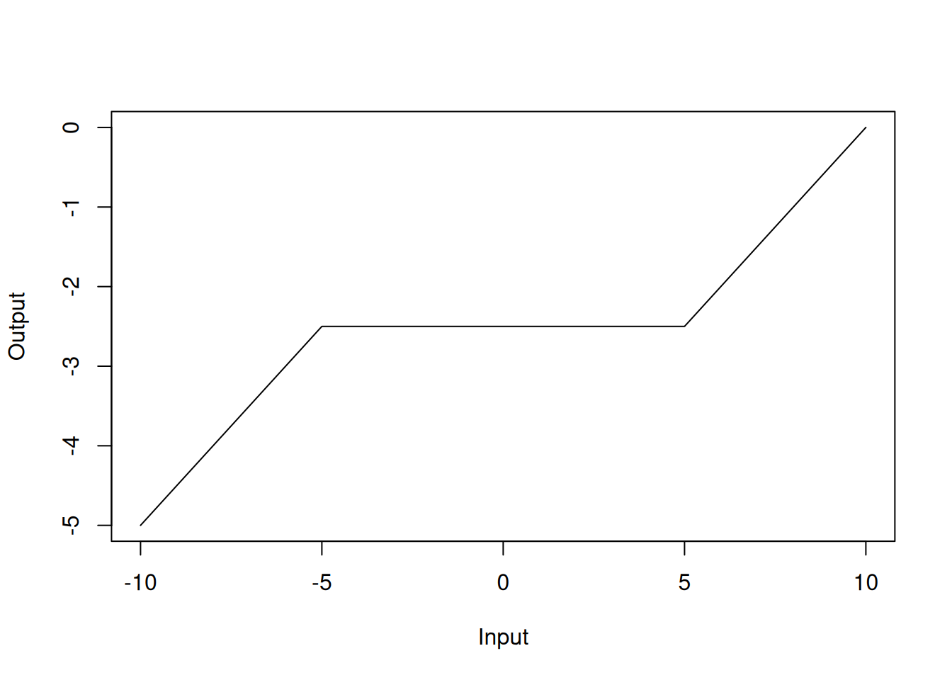
Figure 4.5: MARS model in one dimension
Example
We fit a MARS model to the Boston data set using the earth package within caret.
library(earth)

set.seed(123)
mars.fit.Boston <- train(medv ~ .,
data = Boston,
method = "earth",
trControl = trainControl(method = "cv",
number = 10),
tuneGrid = expand.grid(degree = 1:2,
nprune = 2:10))

summary(mars.fit.Boston)
## Call: earth(x=matrix[506,13], y=c(0.1595,-0.101...), keepxy=TRUE, degree=2,
## nprune=10)
##
## coefficients
## (Intercept) 0.1549343
## h(rm-0.208315) 0.9102939
## h(-1.15797-dis) 15.7464951
## h(lstat- -0.914859) -0.5632729
## h(1.36614-nox) * h(lstat- -0.914859) 0.1849062
## h(0.206892-rm) * h(dis- -1.15797) -0.1600934
## h(rm-0.208315) * h(ptratio-0.0667298) -1.3843533
## h(-0.612548-tax) * h(-0.914859-lstat) 3.8341243
## h(tax- -0.612548) * h(-0.914859-lstat) 2.8353130
##
## Selected 9 of 27 terms, and 6 of 13 predictors (nprune=10)
## Termination condition: Reached nk 27
## Importance: rm, lstat, ptratio, tax, dis, nox, crim-unused, zn-unused, ...
## Number of terms at each degree of interaction: 1 3 5
## GCV 0.137542 RSS 63.93938 GRSq 0.8627298 RSq 0.8733874In the model summary, the h() functions are the hinge functions that are used to create the piecewise linear functions. For instance, h(rm-0.208315) with a coefficient of 0.91 should be interpreted as the hinge function \(\max(0, rm-0.208315)\), which can be visualised as
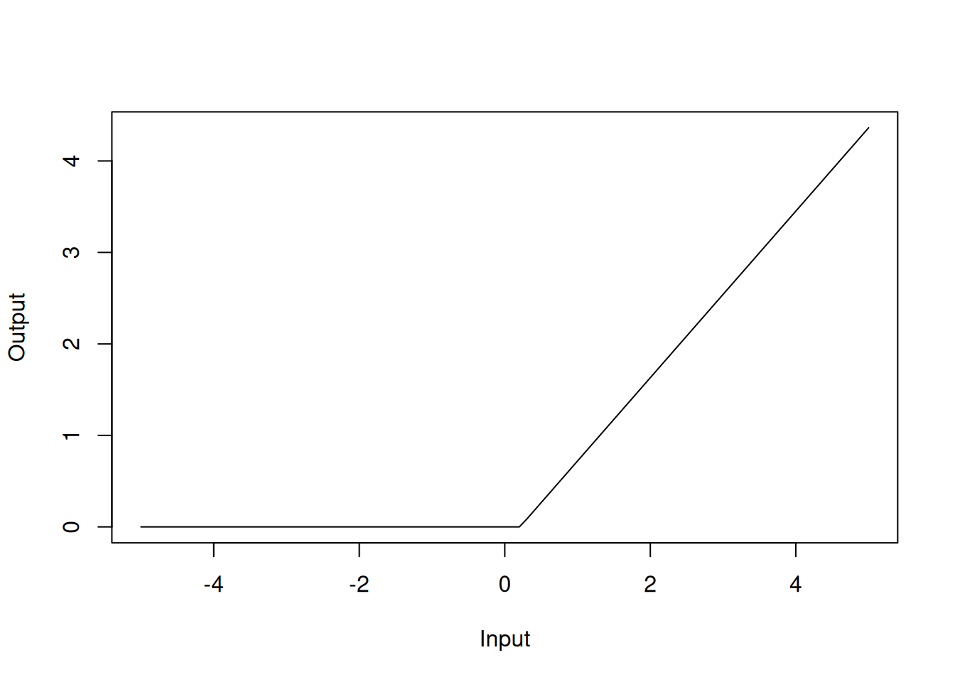
Figure 4.6: Hinge function for rm variable
Similarly, h(-1.15797-dis) with a coefficient of 15.7 should be interpreted as the hinge function \(\max(0, -1.15797-dis)\):
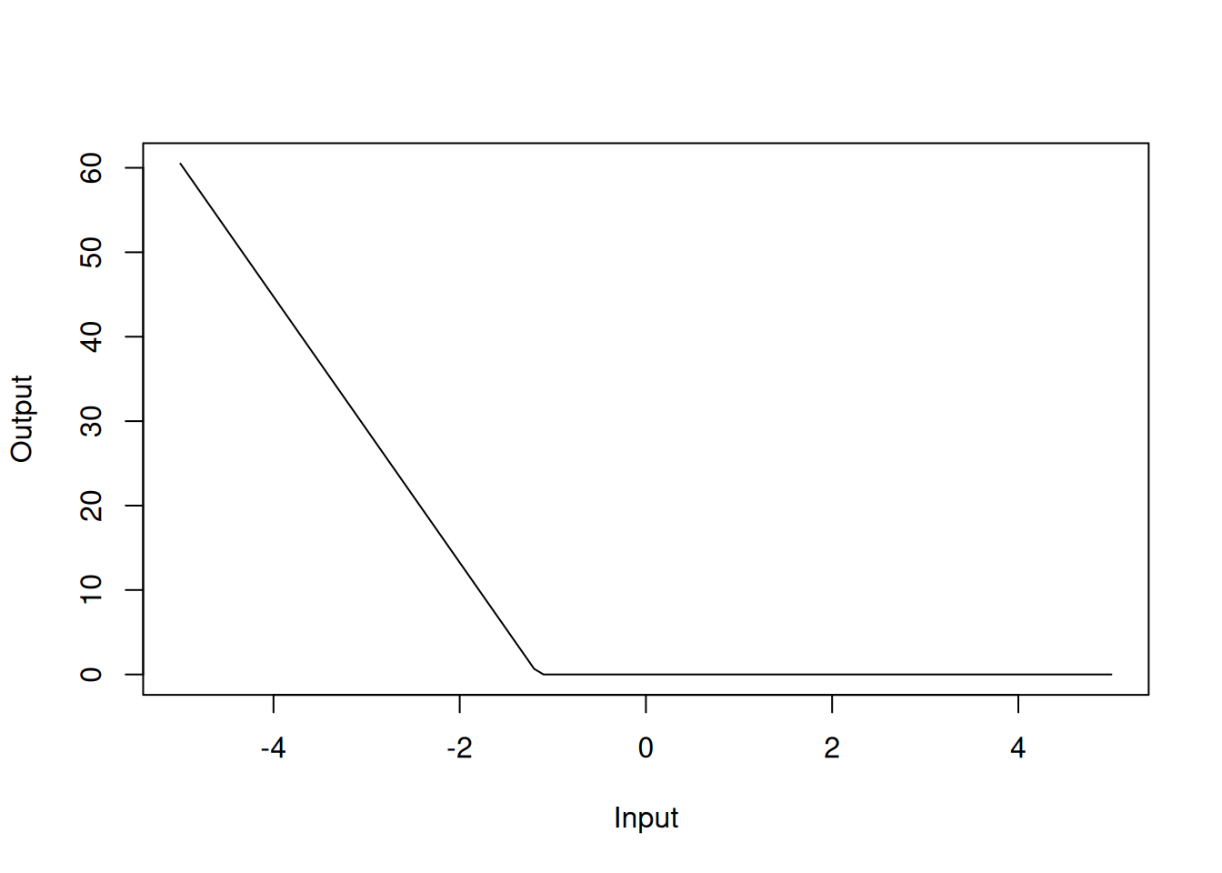
Figure 4.7: Hinge function for dis variable
The MARS model has an RMSE of 0.41. In the model summary, we can see that we have selected 9 of 27 terms, and 6 of the 13 predictors have been used. This means that the MARS model has selected 9 hinge functions for the final model that utilise 6 of the 13 explanatory variables. Like in the standard linear regression case, rm, dis and lstat are important predictors in the MARS model.