Chapter 6 Model Interpretation
A general criticism of machine learning methods is that they are often black boxes: it is difficult to disentangle the influence of one variable from another. This is particularly true for complex models such as random forests and gradient boosting machines where very many simple models have been averaged or aggregated. However, there are several methods that can be used to interpret the results of these models. Model interpretability is crucial in many domains, especially healthcare, finance, and legal applications, where understanding the reasoning behind predictions is often as important as the predictions themselves. Regulatory requirements and ethical considerations often mandate explainable models.
There are several mechanistic insights that we may want to have given a set of data and a model:
Variable importance: Which variables are most important in predicting the outcome?
Variable interactions: Are there interactions between variables that are important in predicting the outcome?
Local interpretability: Given a single observation, can we understand why the model made the prediction it did?
Model structure: What does the model look like? What are the decision rules that the model is using?
In this chapter, we will explore several methods for interpreting the results of a model. We will use the DALEX package to do this. This package provides a unified interface for interpreting the results of a wide variety of models (akin to caret for cross-validation).
6.1 Variable importance
In a simple linear regression model, the coefficients of the model give us a direct measure of the importance of each variable. For example, consider the following linear regression model:
##
## Call:
## lm(formula = mpg ~ ., data = mtcars)
##
## Residuals:
##     Min      1Q  Median      3Q     Max
## -3.4506 -1.6044 -0.1196  1.2193  4.6271
##
## Coefficients:
##             Estimate Std. Error t value Pr(>|t|)
## (Intercept) 12.30337   18.71788   0.657   0.5181
## cyl         -0.11144    1.04502  -0.107   0.9161
## disp         0.01334    0.01786   0.747   0.4635
## hp          -0.02148    0.02177  -0.987   0.3350
## drat         0.78711    1.63537   0.481   0.6353
## wt          -3.71530    1.89441  -1.961   0.0633 .
## qsec         0.82104    0.73084   1.123   0.2739
## vs           0.31776    2.10451   0.151   0.8814
## am           2.52023    2.05665   1.225   0.2340
## gear         0.65541    1.49326   0.439   0.6652
## carb        -0.19942    0.82875  -0.241   0.8122
## ---
## Signif. codes:  0 '***' 0.001 '**' 0.01 '*' 0.05 '.' 0.1 ' ' 1
##
## Residual standard error: 2.65 on 21 degrees of freedom
## Multiple R-squared:  0.869,  Adjusted R-squared:  0.8066
## F-statistic: 13.93 on 10 and 21 DF,  p-value: 3.793e-07
The coefficients of the model give us a direct measure of the importance of each variable. For example, the coefficient of wt is -3.72, which means that for every one unit increase in wt, the predicted value of mpg decreases by 3.72.
It is also straightforward to determine the strength of interactions between variables.
##
## Call:
## lm(formula = mpg ~ . + cyl:disp, data = mtcars)
##
## Residuals:
##     Min      1Q  Median      3Q     Max
## -3.1697 -1.6096 -0.1275  1.1873  3.8355
##
## Coefficients:
##              Estimate Std. Error t value Pr(>|t|)
## (Intercept) 29.976395  18.535141   1.617   0.1215
## cyl         -1.789619   1.183617  -1.512   0.1462
## disp        -0.095947   0.049001  -1.958   0.0643 .
## hp          -0.033409   0.020359  -1.641   0.1164
## drat        -0.541227   1.584761  -0.342   0.7363
## wt          -3.552721   1.717760  -2.068   0.0518 .
## qsec         0.698111   0.664203   1.051   0.3058
## vs           0.828745   1.918957   0.432   0.6705
## am           0.819051   1.997640   0.410   0.6862
## gear         1.554511   1.405425   1.106   0.2818
## carb         0.144212   0.764824   0.189   0.8523
## cyl:disp     0.013762   0.005825   2.363   0.0284 *
## ---
## Signif. codes:  0 '***' 0.001 '**' 0.01 '*' 0.05 '.' 0.1 ' ' 1
##
## Residual standard error: 2.401 on 20 degrees of freedom
## Multiple R-squared:  0.8976, Adjusted R-squared:  0.8413
## F-statistic: 15.94 on 11 and 20 DF,  p-value: 1.441e-07
For example, the coefficient of cyl:disp is 0.01, which means that for every simultaneous unit increase in cyl and disp, the predicted value of mpg increases by 0.01.
6.1.1 Permutation-based variable importance
One way to determine the importance of each variable in a random forest or gradient boosting machine is to use a permutation-based variable importance method. If we are estimating performance metric \(\theta\), this method works as follows:
Fit the model to the data and calculate the model’s performance, \(\widehat{\theta}_0\).
For each variable in turn (\(j=1,\dots,p\)) and for multiple repeats (\(i=1,\dots,M\))
- randomly permute the values of that variable in the data;
- calculate the change in the model’s performance; i.e., \(\widehat{\theta}_0-\widehat{\theta}_j^{(i)}\);
- The importance of each variable is the average change in the model’s performance across all permutations: \[ \text{Importance}(j) = \frac{1}{M} \sum_{i=1}^{M} \left( \widehat{\theta}_0 - \widehat{\theta}_j^{(i)} \right). \]
If a variable is important in predicting the outcome, then permuting the values of that variable should result in a large change in the model’s performance. Conversely, if a variable is not important in predicting the outcome, then permuting the values of that variable should result in a small change in the model’s performance.
The algorithm briefly outlined here is a one-at-a-time method. It is possible that such a method may miss important interactions between variables. There are other methods that can be used to determine the importance of interactions between variables.
Example
Here, we will look at this strategy for a linear regression model and consider its utility in contrast to the more traditional hypothesis tests. Again, instead of relying on a package, we will implement this method ourselves.
# Fit the model
lm_model <- lm(mpg ~ ., data = mtcars)

# Hypothesis test results for each variable
summary(lm_model)
##
## Call:
## lm(formula = mpg ~ ., data = mtcars)
##
## Residuals:
## Min 1Q Median 3Q Max
## -3.4506 -1.6044 -0.1196 1.2193 4.6271
##
## Coefficients:
## Estimate Std. Error t value Pr(>|t|)
## (Intercept) 12.30337 18.71788 0.657 0.5181
## cyl -0.11144 1.04502 -0.107 0.9161
## disp 0.01334 0.01786 0.747 0.4635
## hp -0.02148 0.02177 -0.987 0.3350
## drat 0.78711 1.63537 0.481 0.6353
## wt -3.71530 1.89441 -1.961 0.0633 .
## qsec 0.82104 0.73084 1.123 0.2739
## vs 0.31776 2.10451 0.151 0.8814
## am 2.52023 2.05665 1.225 0.2340
## gear 0.65541 1.49326 0.439 0.6652
## carb -0.19942 0.82875 -0.241 0.8122
## ---
## Signif. codes: 0 '***' 0.001 '**' 0.01 '*' 0.05 '.' 0.1 ' ' 1
##
## Residual standard error: 2.65 on 21 degrees of freedom
## Multiple R-squared: 0.869, Adjusted R-squared: 0.8066
## F-statistic: 13.93 on 10 and 21 DF, p-value: 3.793e-07# Calculate the performance of the model
performance <- summary(lm_model)$r.squared
# Permute the values of each variable in turn
permuted_performance <- sapply(names(mtcars[,-1]),
function(var) {
# Permute the values of the variable
permuted_data <- mtcars
permuted_data[[var]] <- sample(permuted_data[[var]])
# Fit the model to the permuted data
permuted_lm_model <- lm(mpg ~ ., data = permuted_data)
# Calculate the performance of the model
permuted_performance <- summary(permuted_lm_model)$r.squared
# Return the change in performance
return(performance - permuted_performance)
})
# Plot the results
barplot(permuted_performance,
names.arg = names(mtcars[,-1]),
las = 2)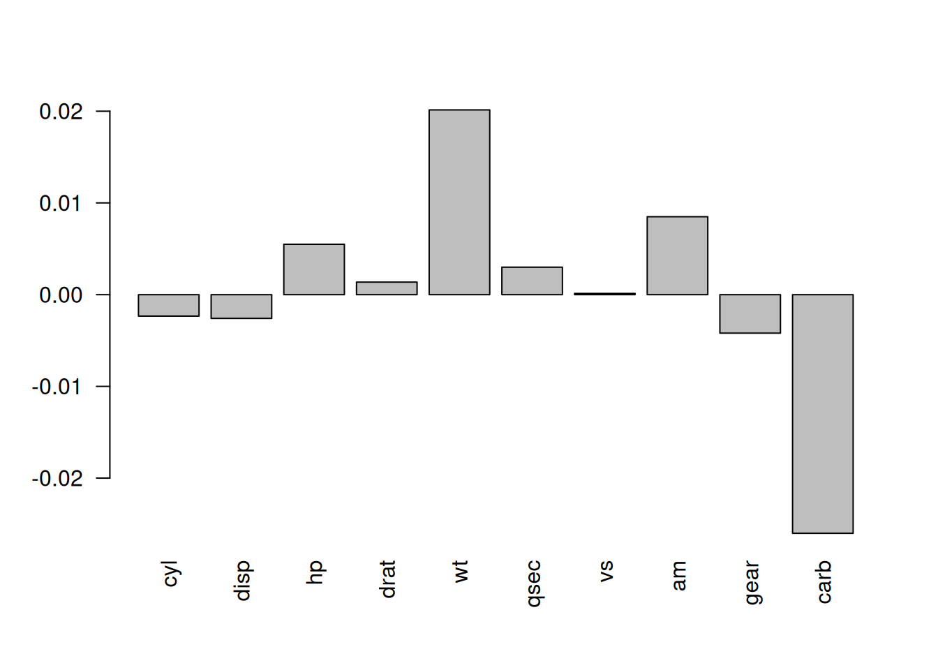
Figure 6.1: The change in performance of the model when the values of each variable are permuted.
There are, of course, packages available in R that will implement this method for you. One such package is DALEX.
Example
Now, we will utilise the DALEX package to determine the importance of each variable in a random forest model for the Boston housing data.
##
## Attaching package: 'ISLR2'
## The following object is masked from 'package:MASS':
##
## Boston## Registered S3 method overwritten by 'DALEX':
## method from
## print.description questionr## Welcome to DALEX (version: 2.5.3).
## Find examples and detailed introduction at: http://ema.drwhy.ai/
## Additional features will be available after installation of: ggpubr.
## Use 'install_dependencies()' to get all suggested dependencies##
## Attaching package: 'DALEX'## The following object is masked from 'package:dplyr':
##
## explain# Fit the random forest model
rf_model <- randomForest(medv ~ ., data = Boston)
# Create an explainer object
explainer <- explain(rf_model,
data = Boston[-14],
y = Boston$medv)## Preparation of a new explainer is initiated
## -> model label : randomForest ( default )
## -> data : 506 rows 13 cols
## -> target variable : 506 values
## -> predict function : yhat.randomForest will be used ( default )
## -> predicted values : No value for predict function target column. ( default )
## -> model_info : package randomForest , ver. 4.7.1.2 , task regression ( default )
## -> predicted values : numerical, min = 6.762044 , mean = 22.55544 , max = 49.12006
## -> residual function : difference between y and yhat ( default )
## -> residuals : numerical, min = -6.271153 , mean = -0.02263104 , max = 8.661072
## A new explainer has been created!# Calculate the importance of each variable
variable_importance <- variable_importance(explainer)
variable_importance## variable mean_dropout_loss label
## 1 _full_model_ 1.405939 randomForest
## 2 medv 1.405939 randomForest
## 3 zn 1.449780 randomForest
## 4 chas 1.477178 randomForest
## 5 rad 1.553602 randomForest
## 6 tax 1.861586 randomForest
## 7 age 1.889014 randomForest
## 8 indus 2.002525 randomForest
## 9 ptratio 2.335230 randomForest
## 10 crim 2.458435 randomForest
## 11 dis 2.563601 randomForest
## 12 nox 2.591746 randomForest
## 13 rm 5.553737 randomForest
## 14 lstat 6.446654 randomForest
## 15 _baseline_ 12.565596 randomForestHere, mean_dropout_loss is the average change in the model’s performance across all permutations. The larger the value, the more important the variable is in predicting the outcome.
6.1.2 Decision tree structure
Another method for interpreting the results of a model is to examine the decision tree structure of the model. Of course, decision trees are far more accessible than other ML methods. As we have seen, there are several packages in R that can be used to visualise the decision tree structure of a model.
In a random forest setting, the decision tree structure of the model can be used to determine the importance of each variable. The importance of each variable is determined by the number of times the variable is used in the decision tree structure.
Example
Here we will use the rpart package to visualise the decision tree structure of a random forest model.
library(randomForest)

# Fit the random forest model
rf_model_cars <- randomForest(mpg ~ .,
                         data = mtcars)

# Extract the decision tree structure of the model
tree <- getTree(rf_model_cars, k = 1, labelVar = TRUE)

# Examine the decision tree structure
tree
## left daughter right daughter split var split point status prediction
## 1 2 3 cyl 5.00 -3 21.69063
## 2 4 5 carb 1.50 -3 27.15333
## 3 6 7 qsec 16.96 -3 16.87059
## 4 0 0 <NA> 0.00 -1 30.82000
## 5 8 9 wt 2.46 -3 25.32000
## 6 10 11 disp 339.00 -3 14.84286
## 7 12 13 carb 1.50 -3 18.29000
## 8 14 15 disp 107.70 -3 27.46667
## 9 0 0 <NA> 0.00 -1 22.10000
## 10 0 0 <NA> 0.00 -1 15.25000
## 11 0 0 <NA> 0.00 -1 14.30000
## 12 0 0 <NA> 0.00 -1 19.75000
## 13 16 17 disp 352.00 -3 17.31667
## 14 0 0 <NA> 0.00 -1 30.40000
## 15 0 0 <NA> 0.00 -1 26.00000
## 16 0 0 <NA> 0.00 -1 16.37500
## 17 0 0 <NA> 0.00 -1 19.20000A function called importance within the randomForest package can be used to identify “important” variables. The measure of importance is the total decrease in node impurities from splitting on the variable, averaged over all trees. For classification, the node impurity is measured by the Gini index. For regression, it is measured by the residual sum of squares.
##      IncNodePurity
## cyl      186.23363
## disp     254.52584
## hp       196.60489
## drat      55.19186
## wt       248.18756
## qsec      27.49346
## vs        24.11108
## am        16.54080
## gear      18.08646
## carb      33.35527
Looking at this measure alone, cyl, disp, hp and wt stand out as the most important as they are allowing the tree algorithm to split into relatively purer branches.
For a random forest model, we can also count how many times variables are used in the decision tree structure.
# Count how many times variables are used in the
# decision tree structure
variable.names(mtcars)[-1]
## [1] "cyl" "disp" "hp" "drat" "wt" "qsec" "vs" "am" "gear" "carb"## [1] 304 856 812 508 811 541 138 109 162 315This might suggest that disp is the most important variable in the model, but it could be that am is the most important but its influence is captured early in the decision tree structure.
Instead, we might count the number of times each variable is used for the first split in a decision tree within the random forest:
# Count how many times each variable is used for the
# first split in a decision tree
first.split <- sapply(1:rf_model_cars$ntree, function(i) {
  rfTree <- getTree(rf_model_cars, k = i, labelVar = TRUE)[1,3]
  variable.names(mtcars)[-1][rfTree]
})

table(first.split)
## first.split
## am cyl disp drat hp qsec vs wt
## 4 81 137 68 82 45 17 66Now, as the first division tends to be the most important in terms of predicting the outcome, we can see that disp and cyl seem to be the most important variables in the model.
6.2 Main effect visualisations
6.2.1 Main effects
A main effect is the effect of a variable on the outcome, while holding all other variables constant. To help us to understand the utility of these let’s consider a situation where we know the true model generating the data.
Example
Here, we have one outcome variable and two explanatory variables. The true model is:
\[ Y = X_1 + X_2^2. \] We will have strongly correlated explanatory variables:
\[\begin{align*} X_1 &\sim \text{Uni}(0, 1), \\ X_2 &= X_1 + \epsilon, \quad \epsilon \sim \text{N}(0, 0.02). \end{align*}\]
Here’s some data for us to work with:
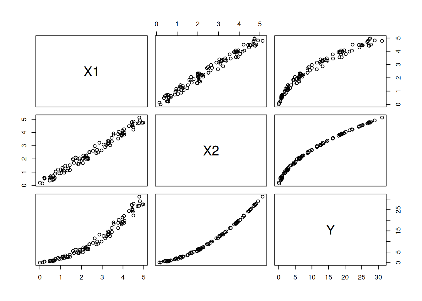
Figure 6.2: The relationship between the variables in the data.
It is trivial to derive the main effect of the model for fixed values of \(X_1\): \[ \begin{aligned} \text{E}[Y|X_1=x_1] &= x_1 + \text{E}[X_2^2|X_1=x_1] \\ &= x_1 + \text{E}[(x_1 + \epsilon)^2]\\ &= x_1 + x_1^2 + \text{E}[\epsilon^2]. \end{aligned} \]
Similarly for fixed values of \(X_2\): \[ \begin{aligned} \text{E}[Y|X_2=x_2] &= \text{E}[X_1|X_2=x_2] + x_2^2 \\&= \text{E}[x_2 - \epsilon] + x_2^2 \\&= x_2 + x_2^2. \end{aligned} \] You will notice in these derivations that we have had to account for the joint distribution of the variables.
Figures 6.3 and 6.4 show the main effects of \(X_1\) and \(X_2\) on \(Y\) respectively (plotted against all the observations).
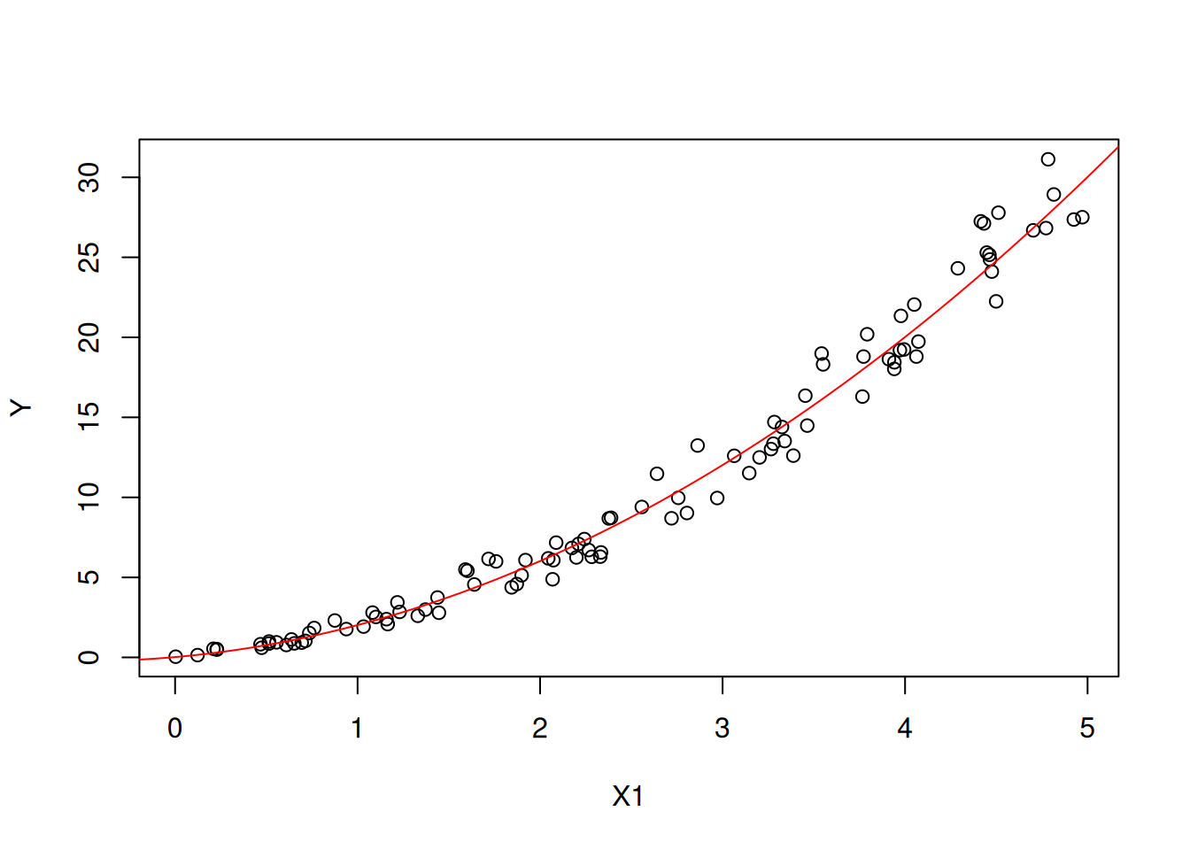
Figure 6.3: The main effect of X1 on Y.
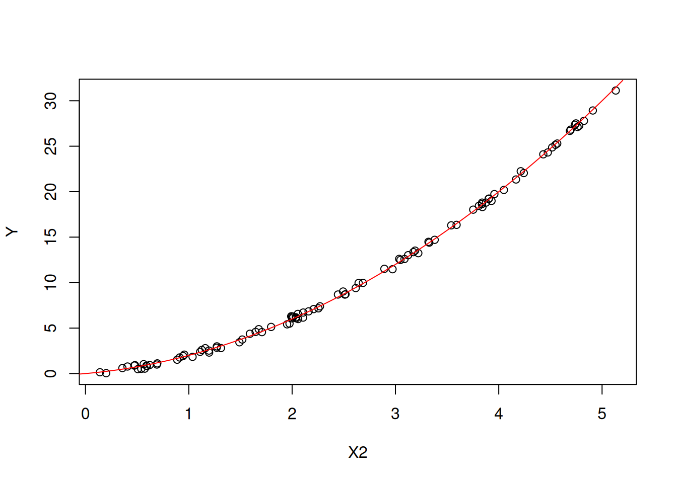
Figure 6.4: The main effect of X2 on Y.
6.2.2 Partial dependence plots
One method for interpreting the results of a model is to use partial dependence plots. A partial dependence plot shows the relationship between a variable and the outcome, while holding all other variables constant. This allows us to see the effect of a variable on the outcome, while controlling for the effects of other variables.
More formally, consider a prediction model \(\widehat{f}(\mathbf{x})\) where \(\mathbf{x} = (x_1, x_2, \ldots, x_p)\) is a vector of \(p\) covariates. Let \(S \subseteq \{1, 2, \ldots, p\}\) be a subset of covariate indices that we are interested in, and let \(C = \{1, 2, \ldots, p\} \setminus S\) be the complement set. We can partition the covariate vector as \(\mathbf{x} = (\mathbf{x}_S, \mathbf{x}_C)\), where \(\mathbf{x}_S\) contains the covariates of interest and \(\mathbf{x}_C\) contains the remaining covariates.
The partial dependence function is defined as the expected value of the model predictions over the marginal distribution of \(\mathbf{x}_C\): \[ \widehat{f}_S(\mathbf{x}_S) = \text{E}_{\mathbf{x}_C}\left[\widehat{f}(\mathbf{x}_S, \mathbf{x}_C)\right] = \int \widehat{f}(\mathbf{x}_S, \mathbf{x}_C) \, p(\mathbf{x}_C) \, d\mathbf{x}_C, \] where \(p(\mathbf{x}_C)\) is the marginal distribution of \(\mathbf{x}_C\).
In practice, the expectation is approximated using a Monte Carlo estimate over the training data. Given a training dataset \(\{(\mathbf{x}^{(i)}, y^{(i)})\}_{i=1}^{n}\), the partial dependence function is estimated as: \[ \widehat{f}_S(\mathbf{x}_S) \approx \frac{1}{n} \sum_{i=1}^{n} \widehat{f}\left(\mathbf{x}_S, \mathbf{x}_C^{(i)}\right). \]
For the common case where \(S\) contains a single covariate \(x_j\), the partial dependence function simplifies to: \[ \widehat{f}_j(x_j) = \frac{1}{n} \sum_{i=1}^{n} \widehat{f}\left(x_1^{(i)}, \ldots, x_{j-1}^{(i)}, x_j, x_{j+1}^{(i)}, \ldots, x_p^{(i)}\right). \]
This formula shows that we evaluate the model at a fixed value of \(x_j\) while averaging over all observed values of the other covariates. It is important to note that partial dependence plots assume that the covariate of interest is independent of the other covariates. When covariates are correlated, the partial dependence function may include predictions at covariate combinations that are unlikely or impossible in the real data, which can lead to misleading interpretations.
Example
Here, we will use the iml package to create a partial dependence plot for the random forest model for the Boston data.
library(iml)

# Create an explainer object
explainer <- Predictor$new(rf_model,
                           data = Boston)

# Create a partial dependence plot for the variable `lstat`
lstat_pd <- FeatureEffect$new(explainer,
                              feature = "lstat",
                              method = 'pdp')

# Plot the partial dependence plot
plot(lstat_pd)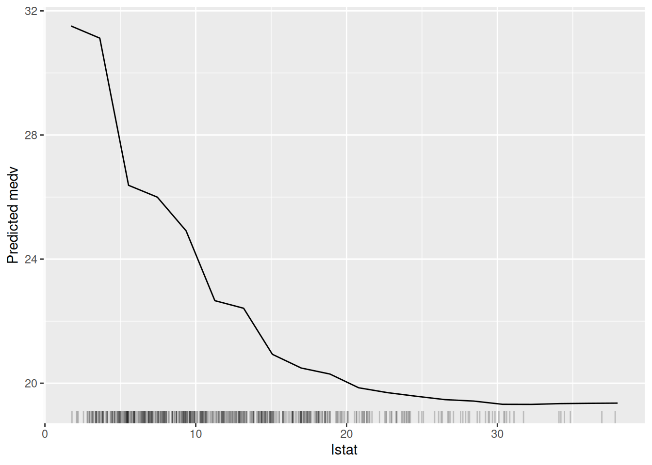
Figure 6.5: The partial dependence plot for the variable lstat.
In Figure 6.5, we can see a clear negative relationship between lstat and medv. As lstat increases, medv decreases. This is consistent with our understanding of the data because lstat is the percentage of lower status of the population, which is likely to be negatively correlated with the median value of owner-occupied homes.
6.2.3 Accumulated local effects
Another method for interpreting the results of a model is to use accumulated local effects (ALE). ALE plots address a key limitation of partial dependence plots: when covariates are correlated, PDPs can extrapolate to unrealistic regions of the covariate space. ALE plots avoid this by considering only local changes in predictions within intervals where data actually exist.
Mathematically, the ALE function for a single covariate \(x_S\) is defined as: \[ \text{ALE}_S(x_S) = \int_{z_{0,S}}^{x_S} \text{E}_{\mathbf{x}_C | x_S = z}\left[\frac{\partial \widehat{f}(\mathbf{x})}{\partial x_S}\right] dz - c, \] where \(z_{0,S}\) is a reference point (typically the minimum value of \(x_S\)), \(\mathbf{x}_C\) denotes the covariates other than \(x_S\), and \(c\) is a centering constant chosen so that the ALE function averages to zero over the distribution of \(x_S\).
In practice, we approximate this integral using a discrete grid. Let \(\{z_{0,S}, z_{1,S}, \ldots, z_{K,S}\}\) be a partition of the range of \(x_S\) into \(K\) intervals. For each interval \([z_{k-1,S}, z_{k,S}]\), let \(n_S(k)\) denote the number of training observations with \(x_S \in [z_{k-1,S}, z_{k,S}]\). The ALE function is then estimated as: \[ \widehat{\text{ALE}}_S(x_S) = \sum_{k=1}^{k_S(x_S)} \frac{1}{n_S(k)} \sum_{i: x_S^{(i)} \in [z_{k-1,S}, z_{k,S}]} \left[\widehat{f}\left(z_{k,S}, \mathbf{x}_C^{(i)}\right) - \widehat{f}\left(z_{k-1,S}, \mathbf{x}_C^{(i)}\right)\right] - c, \] where \(k_S(x_S)\) is the index of the interval containing \(x_S\), and \(c\) is chosen to ensure that the sample mean of \(\widehat{\text{ALE}}_S\) is zero.
The key insight is that, for each observation in an interval, we compute the difference in predictions when \(x_S\) is moved from the lower to the upper boundary of the interval, while keeping all other covariates at their observed values. This local effect is then averaged over all observations in the interval and accumulated across intervals.
The algorithm can be summarised as follows:
- Partitioning the variable’s range:
- Divide the range of the variable into a reasonable number of intervals;
- The number of intervals can influence the smoothness of the ALE plot;
- For each interval, calculate the average value of the variable within that interval.
- Calculating Local Effects:
- For each interval, calculate the difference in the average model prediction between:
- The original data within that interval;
- The data where the variable values within that interval are shifted by a small amount (e.g., half the interval width);
- This difference represents the local effect of the variable within that interval.
- Accumulating Local Effects:
- Start with the lowest interval and calculate the local effect for that interval;
- For each subsequent interval, add the local effect of that interval to the accumulated effect from the previous intervals;
- This gives you the cumulative effect of the variable on the model’s predictions up to that point.
The ALE approach has several advantages over PDPs:
- Unbiased estimation: ALE plots are unbiased even when covariates are correlated, because they only use observed covariate combinations.
- Computational efficiency: ALE plots require fewer model evaluations than PDPs.
- Interpretation: The ALE value at a point \(x_S\) represents the effect of \(x_S\) on the prediction relative to the average effect.
Example
Here, we will again use the iml package to create an ALE plot.
lstat_pd <- FeatureEffect$new(explainer,
                              feature = "lstat",
                              method = 'ale')

# Plot the partial dependence plot
plot(lstat_pd)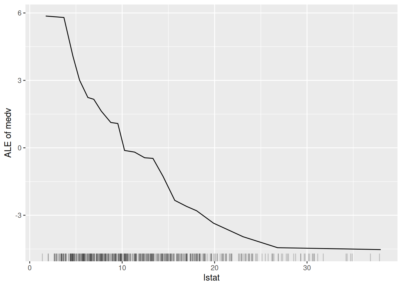
Figure 6.6: The ALE plot for the variable lstat.
Figure 6.6 is very similar to Figure 6.5. This is perhaps because there is not a great amount of interaction between lstat and the other variables in the model. However, the ALE plot is more interpretable than the partial dependence plot because it shows the difference in predictions when lstat is changed, rather than the average prediction itself.