Using Categorical Covariates with AddiVortes

This vignette explains how AddiVortes handles categorical covariates — variables that take a discrete set of named levels, such as region, product type, or treatment group. Because Voronoi tessellations require numerical distances between points, categorical variables must first be converted to numbers. AddiVortes does this automatically using one-hot encoding, and this vignette explains the encoding in detail.

1. What is One-Hot Encoding?

A categorical variable with d distinct levels cannot be treated as a number because there is no natural ordering or magnitude between categories. For example, assigning “North” = 1, “South” = 2, “East” = 3, “West” = 4 would incorrectly imply that “West” is four times “North”.

One-hot encoding converts a categorical variable with d levels into d − 1 binary (0/1) indicator columns. One level is chosen as the reference level (by convention, the first level in alphabetical order), and the remaining d − 1 levels each receive their own column:

Level	`region_North`	`region_South`	`region_West`
East	0	0	0
North	1	0	0
South	0	1	0
West	0	0	1

The reference level (“East” here, as the alphabetically first) is represented by all zeros. Using d − 1 rather than d columns avoids perfect collinearity while retaining full information about group membership.

AddiVortes applies this encoding automatically to any column in x that is of type character or factor. You do not need to pre-process your data.

2. The `catScaling` Parameter

After one-hot encoding, each indicator column takes values 0 or 1, while continuous covariates are normalised to the range [−0.5, 0.5]. If catScaling = 1 (the default), the binary jump from 0 to 1 has a magnitude comparable to the full range of a normalised continuous covariate, giving categorical and continuous covariates roughly equal influence on the Voronoi tessellation distances.

You can adjust this with the catScaling argument:

catScaling > 1: gives categorical differences more weight than continuous differences.
catScaling < 1: gives categorical differences less weight, making the model rely more heavily on continuous covariates.

The column name for each binary indicator follows the pattern <original_column>_<level>. For example, a column region with levels "East", "North", "South", "West" produces columns region_North, region_South, region_West (with "East" as reference).

3. A Synthetic Example

We create a dataset of 400 observations with two continuous covariates and two categorical covariates. The response variable depends on all four:

library(AddiVortes)

set.seed(123)
n <- 400

x <- data.frame(
  age     = rnorm(n, mean = 40, sd = 10),
  income  = runif(n, 20, 120),               # income in thousands
  region  = sample(c("East", "North", "South", "West"), n, replace = TRUE),
  product = sample(c("Basic", "Premium", "Deluxe"), n, replace = TRUE),
  stringsAsFactors = FALSE
)

# True response: depends on continuous and categorical variables
region_effect  <- ifelse(x$region  == "North",  5,
                  ifelse(x$region  == "South", -5, 0))
product_effect <- ifelse(x$product == "Premium", 10,
                  ifelse(x$product == "Deluxe",  20, 0))

y <- 0.3 * x$age +
     0.1 * x$income +
     region_effect  +
     product_effect +
     rnorm(n, sd = 3)

Note that region has 4 levels and product has 3 levels. When passed to AddiVortes as character columns, they will be encoded as 3 and 2 binary columns respectively — for a total of 5 extra columns alongside the 2 continuous covariates.

4. Inspecting the Encoding

We can call the internal encoding function directly to see exactly what the encoded matrix looks like before fitting the model.

# Show the first few rows of x before encoding
head(x, 5)
#>        age   income region product
#> 1 34.39524 67.06818   East Premium
#> 2 37.69823 56.58455   West   Basic
#> 3 55.58708 32.12721  North Premium
#> 4 40.70508 24.69937   East Premium
#> 5 41.29288 46.27963   East   Basic

# Manually inspect the encoding applied by AddiVortes
enc_result <- AddiVortes:::encodeCategories_internal(x, catScaling = 1)
head(enc_result$encoded, 5)
#>           age   income region_North region_South region_West product_Deluxe
#> [1,] 34.39524 67.06818            0            0           0              0
#> [2,] 37.69823 56.58455            0            0           1              0
#> [3,] 55.58708 32.12721            1            0           0              0
#> [4,] 40.70508 24.69937            0            0           0              0
#> [5,] 41.29288 46.27963            0            0           0              0
#>      product_Premium
#> [1,]               1
#> [2,]               0
#> [3,]               1
#> [4,]               1
#> [5,]               0

The columns produced are: - age and income (unchanged continuous columns) - region_North, region_South, region_West (3 indicators; “East” is the reference) - product_Deluxe, product_Premium (2 indicators; “Basic” is the reference)

All binary columns take values 0 or catScaling (here 1). When catScaling = 1 all indicator columns and the continuous columns span a comparable range inside the model.

5. Fitting the Model

Fitting the model is identical to the standard workflow — simply pass the data frame with character or factor columns directly. AddiVortes handles the encoding internally.

# Split into training and test sets
set.seed(42)
train_idx <- sample(n, 300)

x_train <- x[ train_idx, ]
y_train <- y[ train_idx]
x_test  <- x[-train_idx, ]
y_test  <- y[-train_idx]

fit <- AddiVortes(
  y            = y_train,
  x            = x_train,
  m            = 50,
  totalMCMCIter = 500,
  mcmcBurnIn   = 100,
  catScaling   = 1,         # default: binary columns span [0, 1]
  showProgress = FALSE
)

cat("In-sample RMSE:", round(fit$inSampleRmse, 3), "\n")
#> In-sample RMSE: 2.393

# The catEncoding field records how the encoding was built
cat("\nReference levels used:\n")
#> 
#> Reference levels used:
for (j in fit$catEncoding$catColIndices) {
  orig_col <- fit$catEncoding$origColNames[j]
  ref_lev  <- fit$catEncoding$colEncodings[[j]]$levels[1]
  all_lev  <- fit$catEncoding$colEncodings[[j]]$levels
  cat(" ", orig_col, ": reference =", ref_lev,
      "| all levels:", paste(all_lev, collapse = ", "), "\n")
}
#>   region : reference = East | all levels: East, North, South, West 
#>   product : reference = Basic | all levels: Basic, Deluxe, Premium

The encoding metadata is stored in fit$catEncoding and is automatically used when making predictions, so new data passed to predict() is encoded with exactly the same reference levels.

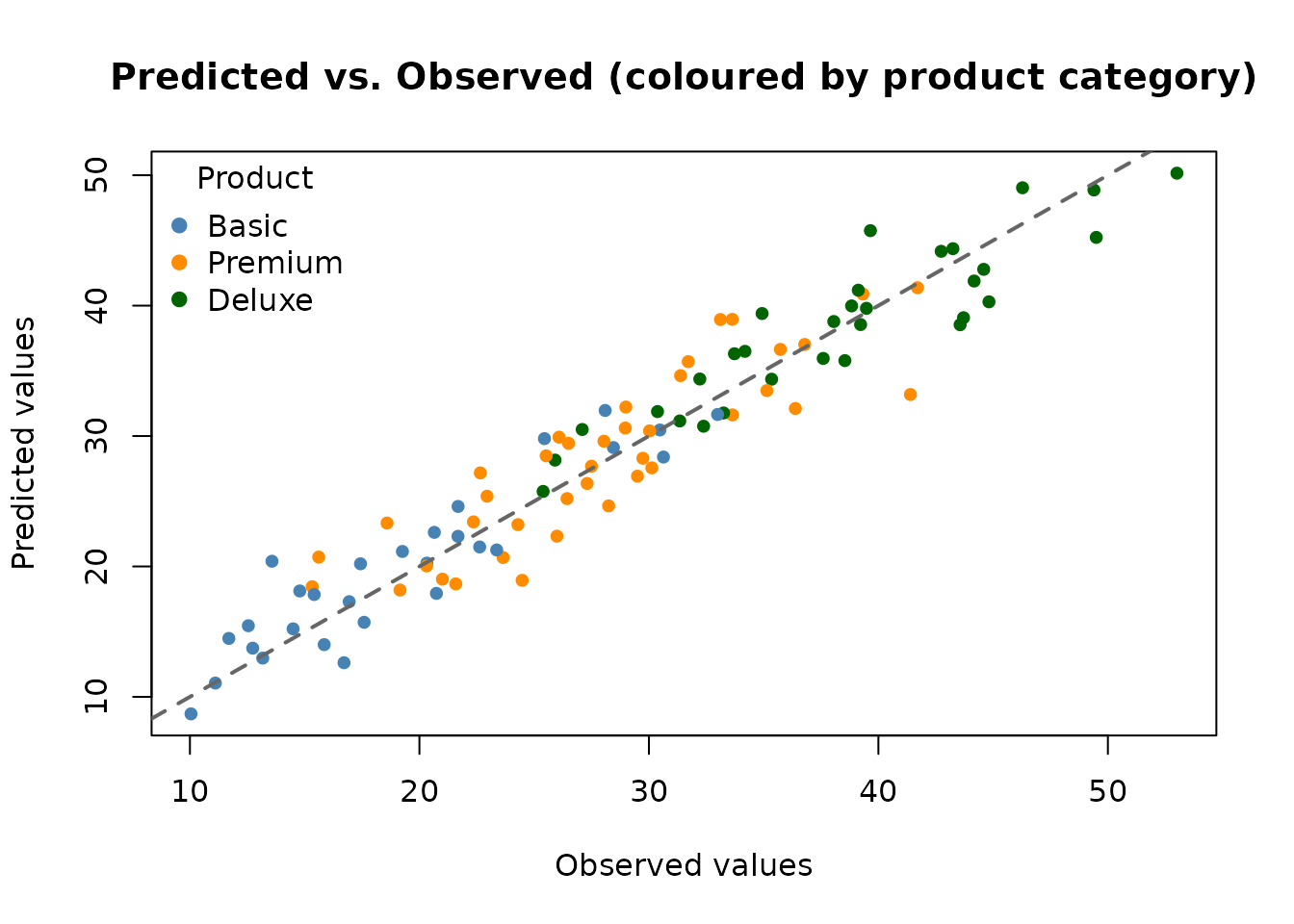
6. Making Predictions

Predictions on new data work in the usual way. If the new data contains the same categorical levels as the training data, the encoding is applied consistently.

preds <- predict(fit, x_test, showProgress = FALSE)

rmse_test <- sqrt(mean((y_test - preds)^2))
cat("Test RMSE:", round(rmse_test, 3), "\n")
#> Test RMSE: 2.883

# Colour observations by product category
prod_cols <- c("Basic" = "steelblue", "Premium" = "darkorange", "Deluxe" = "darkgreen")
point_cols <- prod_cols[x_test$product]

plot(y_test, preds,
     col  = point_cols, pch = 19, cex = 0.8,
     xlab = "Observed values",
     ylab = "Predicted values",
     main = "Predicted vs. Observed (coloured by product category)")
abline(0, 1, lwd = 2, lty = 2, col = "grey40")
legend("topleft",
       legend = names(prod_cols),
       col    = prod_cols,
       pch    = 19, title = "Product", bty = "n")

7. Handling Unseen Category Levels

At prediction time, if a new observation contains a category level that was not seen during training, AddiVortes treats it as the reference level (all binary indicators set to zero). This is a sensible default: the model cannot infer anything about a previously unseen level and falls back to the baseline.

# Create a test point with an unseen product level "Luxury"
x_new <- data.frame(
  age     = 45,
  income  = 80,
  region  = "North",
  product = "Luxury",   # unseen level
  stringsAsFactors = FALSE
)

pred_new <- predict(fit, x_new, showProgress = FALSE)

cat("Prediction for unseen category 'Luxury' (treated as 'Basic'):",
    round(pred_new, 3), "\n")
#> Prediction for unseen category 'Luxury' (treated as 'Basic'): 25.783

8. Effect of `catScaling`

The catScaling parameter controls how much influence categorical differences have in the distance calculations. Here we fit two models — one with catScaling = 1 (equal weight) and one with catScaling = 2 (double weight for categorical differences) — and compare their test RMSEs.

fit_cs2 <- AddiVortes(
  y            = y_train,
  x            = x_train,
  m            = 50,
  totalMCMCIter = 500,
  mcmcBurnIn   = 100,
  catScaling   = 2,         # give categorical differences twice as much weight
  showProgress = FALSE
)

preds_cs2 <- predict(fit_cs2, x_test, showProgress = FALSE)

cat("Test RMSE (catScaling = 1):", round(rmse_test, 3), "\n")
#> Test RMSE (catScaling = 1): 2.883
cat("Test RMSE (catScaling = 2):", round(sqrt(mean((y_test - preds_cs2)^2)), 3), "\n")
#> Test RMSE (catScaling = 2): 2.955

In this example, the true response has substantial category effects (up to ±20 units for product type) relative to the continuous effects, so increasing catScaling may help the model focus more on categorical group membership.

9. Summary of Key Points

Pass character or factor columns directly in the covariate data frame; AddiVortes encodes them automatically.
One-hot encoding: a categorical variable with d levels is converted to d − 1 binary (0/1) indicator columns.
The reference level is the alphabetically first level; all its indicators are zero.
Indicator columns are named <original_column>_<level> (e.g. product_Premium).
catScaling (default 1) controls the weight given to categorical differences relative to continuous differences. Increase it to give categories more influence; decrease it to give them less.
The encoding metadata is stored in fit$catEncoding and applied automatically to new data in predict().
Unseen category levels at prediction time are treated as the reference level.

John Paul Gosling and Adam Stone

2026-03-12

1. What is One-Hot Encoding?

2. The `catScaling` Parameter

3. A Synthetic Example

4. Inspecting the Encoding

5. Fitting the Model

6. Making Predictions

7. Handling Unseen Category Levels

8. Effect of `catScaling`

9. Summary of Key Points

Using Categorical Covariates with AddiVortes

John Paul Gosling and Adam Stone

2026-03-12

1. What is One-Hot Encoding?

2. The catScaling Parameter

3. A Synthetic Example

4. Inspecting the Encoding

5. Fitting the Model

6. Making Predictions

7. Handling Unseen Category Levels

8. Effect of catScaling

9. Summary of Key Points

2. The `catScaling` Parameter

8. Effect of `catScaling`