Machine Learning with AddiVortes: A Bayesian Alternative to BART

John Paul Gosling and Adam Stone

2025-09-09

This vignette provides a comprehensive example of how to use the AddiVortes package for machine learning regression tasks. AddiVortes offers a Bayesian alternative to BART (Bayesian Additive Regression Trees), using Voronoi tessellations for spatial partitioning. We will walk through loading data, training a regression model, and making predictions on a test set using this powerful non-parametric Bayesian approach.

1. Loading the Package and Data

First, we load the AddiVortes package. For this example, we will use the well-known Boston Housing dataset.

# Load the package
require(AddiVortes)

# Load the Boston Housing dataset from a URL
Boston <- read.csv(paste0("https://raw.githubusercontent.com/anonymous2738/",
                          "AddiVortesAlgorithm/DataSets/BostonHousing_Data.csv"))


# Separate predictors (X) and the response variable (Y)
X_Boston <- as.matrix(Boston[, 2:14])
Y_Boston <- as.numeric(as.matrix(Boston[, 15]))

# Clean up the environment
rm(Boston)

2. Preparing the Data

To evaluate the model’s performance, we need to split the data into a training set and a testing set. We will use a standard 5/6 split for training and 1/6 for testing.

n <- length(Y_Boston)

# Set a seed for reproducibility
set.seed(1025)

# Create a training set containing 5/6 of the data
TrainSet <- sort(sample.int(n, 5 * n / 6))

# The remaining data will be our test set
TestSet <- setdiff(1:n, TrainSet)

3. Training the Model

Now we can run the main AddiVortes function on our training data. We will specify several parameters for the algorithm, such as the number of iterations and trees.

# Run the AddiVortes algorithm on the training data
results <- AddiVortes(y = Y_Boston[TrainSet], 
                      x = X_Boston[TrainSet, ],
                      m = 200, 
                      totalMCMCIter = 2000, 
                      mcmcBurnIn = 200, 
                      nu = 6, 
                      q = 0.85, 
                      k = 3, 
                      sd = 0.8, 
                      omega = 3, 
                      lambdaRate = 25,
                      IntialSigma = "Linear",
                      showProgress = FALSE)

4. Making Predictions and Evaluating Performance

With a trained model object, we can now make predictions on our unseen test data. We will then calculate the Root Mean Squared Error (RMSE) to see how well the model performed.

# Generate predictions on the test set
preds <- predict(results,
                 X_Boston[TestSet, ],
                 showProgress = FALSE)

# The RMSE is contained in the results object
cat("In-Sample RMSE:", results$inSampleRmse, "\n")
#> In-Sample RMSE: 1.185435

# Calculate the Root Mean Squared Error (RMSE) for the test set
rmse <- sqrt(mean((Y_Boston[TestSet] - preds)^2))
cat("Test Set RMSE:", rmse, "\n")
#> Test Set RMSE: 3.060899

5. Visualising the Results

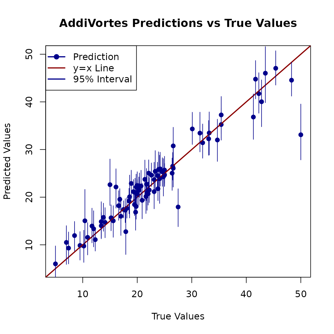
Finally, a good way to assess the model is to plot the predicted values against the true values. For a perfect model, all points would lie on the equality line (y = x). We will also plot the prediction intervals to visualise the model’s uncertainty.

# Plot true values vs. predicted values
plot(Y_Boston[TestSet],
     preds,
     xlab = "True Values",
     ylab = "Predicted Values",
     main = "AddiVortes Predictions vs True Values",
     xlim = range(c(Y_Boston[TestSet], preds)),
     ylim = range(c(Y_Boston[TestSet], preds)),
     pch = 19, col = "darkblue"
)

# Add the line of equality (y = x) for reference
abline(a = 0, b = 1, col = "darkred", lwd = 2)

# Get quantile predictions to create error bars/intervals
preds_quantile <- predict(results,
                          X_Boston[TestSet, ],
                          "quantile",
                          showProgress = FALSE)

# Add error segments for each prediction
for (i in 1:nrow(preds_quantile)) {
  segments(Y_Boston[TestSet][i], preds_quantile[i, 1],
           Y_Boston[TestSet][i], preds_quantile[i, 2],
           col = "darkblue", lwd = 1
  )
}
legend("topleft", legend=c("Prediction", "y=x Line", "95% Interval"), 
       col=c("darkblue", "darkred", "darkblue"),
       lty=1, pch=c(19, NA, NA), lwd=2)